How the Noise node works

Nodes

The Noise* nodes works like other Uniform* nodes: they produces a deterministic noisy signal which can be made available to the shader when attached to the associated Render or Compute.

In the case of the NoiseFloat, the shader obtains a float sample corresponding to the noise signal at a given time t. Similarly, NoiseVec2, NoiseVec3 and NoiseVec4 will respectively provides a vec2, vec3 and vec4 to the shader, where each component of the vector provides a different signal with the same parameters.

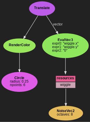
The node themselves can not be used to create advanced patterns/fractals or even display a waveform within a shader because there is only one random value at a given time. On the other hand, it can typically be used to “wiggle” an object or a parameter.

A wiggle effect on an hexagon

Code

Graph

import pynopegl as ngl


@ngl.scene()
def wiggle(cfg: ngl.SceneCfg):
    cfg.aspect_ratio = (1, 1)
    cfg.duration = 3

    geometry = ngl.Circle(radius=0.25, npoints=6)
    render = ngl.RenderColor(geometry=geometry)

    # Extend 2-dimensional noise into a vec3 for the Translate node using EvalVec3
    translate = ngl.EvalVec3("wiggle.x", "wiggle.y", "0")
    translate.update_resources(wiggle=ngl.NoiseVec2(octaves=8))

    return ngl.Translate(render, vector=translate)

This mechanism could be implemented fully in GPU, but a GPU hash function can be costly, difficult to get right, and hardly shared between pipelines. Having the Noise builtin and CPU side allows a fast random generation as well as sharing the signal between different branches. It gives shader a simple and efficient source of noise that can be used in various creative situations.

Seed

Behind the scene, there is only one signal of noise generated. In order to make different signals, the Noise*.seed parameter can be used. In practice, the seed acts as an offsetting of the time t (in seconds), meaning you likely want to keep seeds relatively apart from each other.

That same mechanism is used internally to decorrelate components in the NoiseVec2, NoiseVec3 and NoiseVec4 nodes, using the seed parameter only as base seed (the first component).

Algorithm

Random source

At the most elementary level, we generate random values from x-axis values. The hashing function we use is lowbias32 from Chris Wellons, converted to a float between 0.0 and 1.0. This hashing function makes sure that for a given integer (the lattice / integer coordinate), we will always provide the same float value with a uniform distribution.

We can not use a PRNG because it relies on a state where we need determinism (for one coordinate, we always want the same random value). LCG are a sub-classes of PRNG where the state is actually the returned value. But even then, we can not re-use the previously returned value since we need seeking; that is the ability to get the random value associated with our integer coordinate. Trying to feed a PRNG/LCG with our coordinate instead of the expected state would be equivalent to changing the seed at every call, and this creates an important bias in the random distribution. This is the reason why we need integer hashing instead. lowbias32 has been derived from an advanced generator and was evaluated to be extremely good.

Random signal

Using these random values as “key frames” and interpolating between them would give us a Value Noise, as illustrated below:

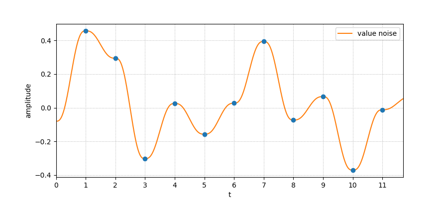
The patterns generated in such a way are not desirable due to the variation in frequencies: when points are close the frequency is low, and can suddenly fluctuates. So instead of using the random values as the noise signal itself, we interpret them as gradient: this is the Gradient Noise, used in the popular Perlin Noise. In our case, since we use a 1D signal, it looks like the following:

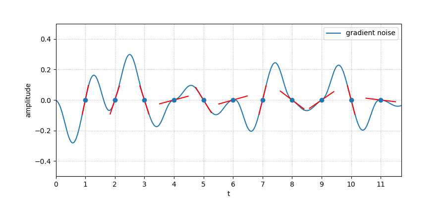
Random values of 0 and 1 (the output of the hash function rescaled into a float) respectively correspond to a tilt of -45° (-π/4) and 45° (π/4).

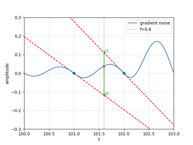
The interpolation between 2 gradient points works that way: for a given time value t between 2 gradients, we obtain two y-axis coordinates by extending the line of each of these gradients. The signal value at t lies somewhere between these 2 points: y0 and y1 are the boundaries of the interpolation. f is used to represent the x-axis distance between t and each lattice (where the gradients are located); we use it as an amount for the non-linear interpolation (see next section for the formulas) to get the finale value.

Note: one important property of the gradient noise is that it passes through 0 at every lattice / cycle.

Interpolants

The two common interpolation functions are:

1. the Cubic Hermite curve, f(t)=3t²-2t³ (typically used in GLSL smoothstep()) initially used by Ken Perlin in his first Perlin Noise implementation

2. the more modern (and complex) quintic curve f(t)=6t⁵-15t⁴+10t³ introduced in 2002 by Ken Perlin in his proposed improved version of the Perlin Noise, in order to address discontinuities in the 2nd order derivatives f"(t).

Both functions are available in the Noise*.interpolant parameter, along with a linear interpolation f(t)=t which can be used for debugging purpose. It is not recommended to use that one for another purpose because it will cause an undesired output (flat curve) if the gradients are oriented the same.

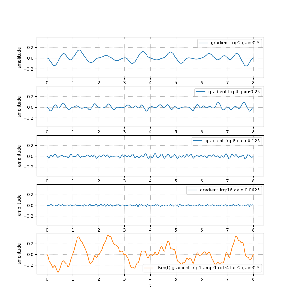
Accumulation

The finale noise is generated using a form of fractional Brownian motion, which basically means multiple layers of gradient noise are added together to create a refined pattern. The parameter controlling the number of layers accumulated is Noise*.octaves.

With the standard parameters, each octave will see its frequency double (Noise*.lacunarity=2) and its amplitude halved (Noise*.gain=½) from the previous one. The gain is also known as persistence, and in its mathematical form derived from the Hurst exponent. This gain/persistence/Hurst notion refers to the same thing, which is the “memory” between octaves, or self-similarity.

As stated earlier, the gradient noise crosses 0 on every lattice. Even when cumulated with other frequencies, this pattern will remain if the lacunarity is an integer. Using 1.98 instead of 2.0 can prevent this (of course, with more than one octave).